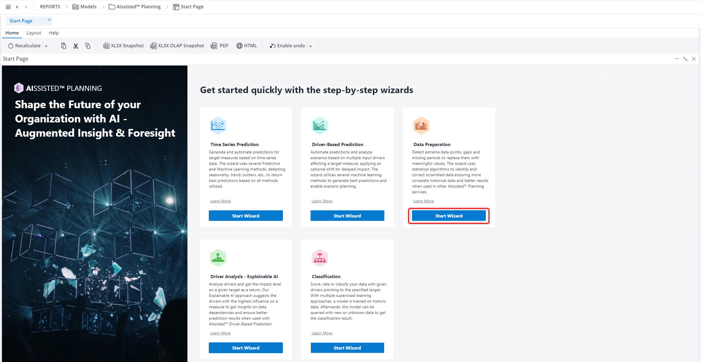
Accurate predictions with machine learning and AI are heavily dependent on the quality of source data. Incomplete or incorrect data will almost always lead to poor-quality prediction results, so before running predictions, it is wise to ensure data quality. The Data Preparation Wizard is designed to help do this in a few steps. Start by choosing the Data Preparation Wizard from the Start Page.

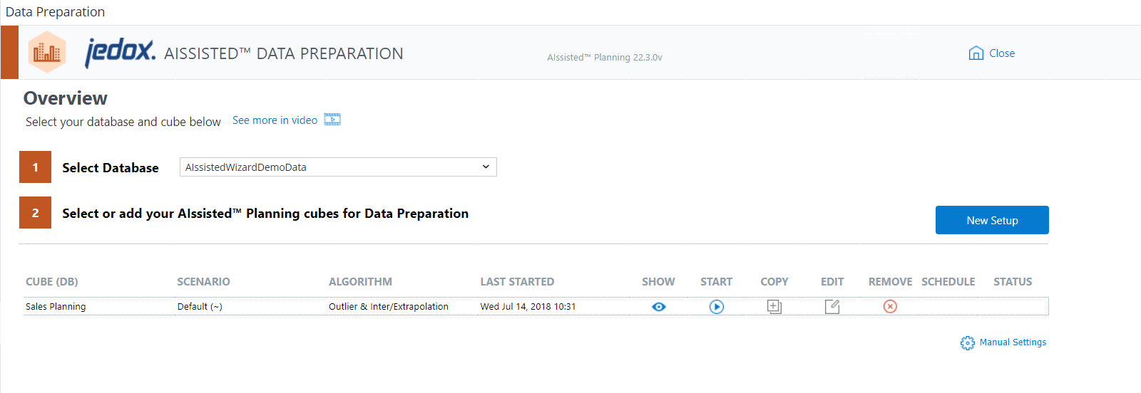
The Data Preparation Overview shows the databases and cubes equipped with the data preparation scenario. Choose a database, and the cubes with information relevant to their scenario will appear below.

The fields of the Data Preparation Overview are described below:

Field	Description
Select Database	A dropdown of all databases stored in your Jedox instance. The database is your native work environment populated with custom data. We also provide demo data to allow you to familiarize yourself with driver analysis functionality outside of your own work environment.
CUBE (DB)	You may choose any cube for data preparation purposes, so long as it has at least three dimensions it can utilize as the Time, Version, and Measure dimensions. The database is your native work environment populated with custom data. We also provide demo data to allow you to familiarize yourself with data preparation functionality outside of your own work environment.
SCENARIO	Shows the saved scenarios for each cube. This can be used to create different data preparation setups for the same cube.
ALGORITHM	AIssisted™ Data Preparation uses a number of different algorithms. Each calculates outlier detection and interpolation in a different way. It can also expand and add missing data points to the beginning or end of limited data sets with extrapolation. Unlike the other wizards, the Data Preparation Wizard cannot offer a Best algorithm choice, because there is no possible accuracy to compare. The wizard provides the best default scenario and the user can change these algorithms according to his needs and specific source data. For more information, please see the Algorithm Presentation document in the Marketplace listing and the Documentation in the Report Designer/AIssisted™ Planning/Files area.
LAST STARTED	Shows the last time each cube's scenario started.
INPUT range	Shows the start date and end date of the time period undergoing the data preparation.
START (button)	Runs data preparation for your cube with existing settings.
COPY (button)	Allows you to copy an existing scenario by selecting it from the list of the "Copy Scenario" dialog, or add a new scenario, which will then appear in the "Scenario" list for selection. Click the Save Changes button to confirm the task.
EDIT (button)	Allows you to adjust the input data of the cube (e.g. change the preparation range, use a different algorithm, or chose different dimensions/elements).
REMOVE (button)	Removes the AIssisted™ Data Preparation scenario from the cube. The default settings for this will also delete the versions with the suggested values. If you would like to keep these versions, uncheck the option in confirmation prompt pop-up.
PREVIEW (button)	Shows a preview of the populated values and compares the actual data with your suggested data.
STATUS (button)	Displays the status of the Integrator job after you start it. To see eventual changes, click the refresh icon in the "Status" column. Once finished, it will show a different icon with the results. Click on the icon for more information.
New Setup (button)	Adds AIssisted™ Data Preparation scenario to a cube.
Manual Settings (button)	Used to change prediction setups and scenarios without entering the wizard itself. Read more about it in Manual Settings for AIssisted™ Planning.

Click New Setup to create a new data preparation scenario. The wizard will guide you through the necessary steps.

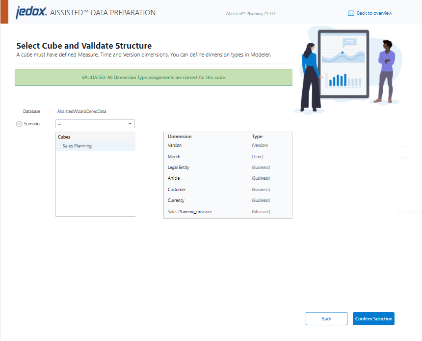
The selected database is shown along with a dropdown menu of scenarios and a list of available cubes stored within the database.

The "Cubes" list allows you to choose the particular cube on which you would like to perform data preparation analysis. The selection will indicate with a green or red message box whether the selected cube is validated for the analysis, i.e., whether it has the required dimensions. A validated cube must have a Time dimension, a Version dimension, and a Measure dimension. Click the Advanced Setting button to access the dimension type assignments.

It is recommended to not use dimensions that contain special characters in their names (e.g. , / $), as these can cause problems when using the wizard.

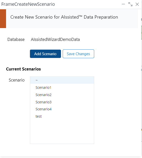
The "Scenario" combobox gives you the option to save more than one scenario per cube. Select your scenario from the dropdown menu or click the + to open the "Create New Scenario" dialog. There you can add a new scenario, which will then appear in the "Scenario" list for selection. Click the Save Changes button to confirm the task.

Once you have selected a validated cube, click Confirm Selection and then click Next.

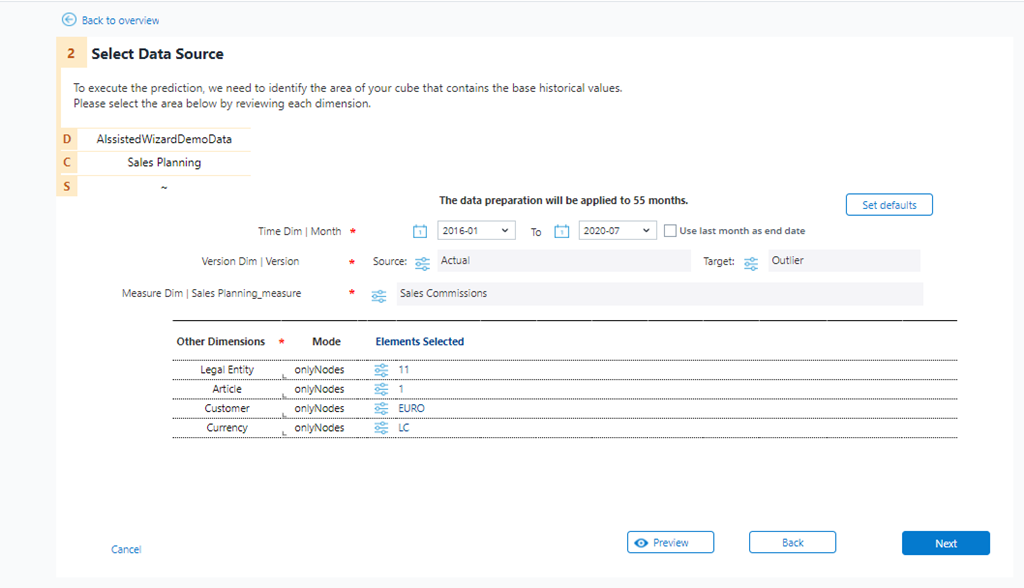
You have selected your cube. Now you must narrow your selection to a specific data slice.

The components of this slice are the Time, Version, and Measure dimensions, located in the upper portion of the wizard. Check the box next to "Use last month as end date" in order to choose the last finished month as the end of the input range instead of using a fixed range. This feature allows you to fully automate the process of data preparation for your monthly planning.

The Other Dimensions, found in the lower portion, will further fine-tune your selection.

The Set defaults button dynamically selects the dimensions and elements based on the layout of your data. You may also select your source material manually. Simply select the start and end Time dimensions from the comboboxes, then click the adjustment icons ( ) to select the rest of your source material, which can include multiple elements per dimension, with the exception of the Time dimensions.

The mode setting for other dimensions has two options: onlyNodes and onlyBases. This sets whether the data preparation will use data at the consolidated (node) level or at the base level. If the mode is set to onlyNodes, the prediction results will be splashed down to the base level using the same distribution as the last period of actual data. When choosing onlyBases, consider how many base level elements each of your consolidated elements has. If an element has 3000 base level elements, choosing onlyBases may cause the volume to be too large, which might cause the setup to fail. It is recommended to break the setup into several different scenarios.

When analyzing data, onlyNodes uses exactly the elements you specified for the prediction. For example, if you specify "All Regions" in the Region dimension, a time series from the consolidated element "All Regions" is used as the source data. In contrast, using onlyBases causes the prediction to be calculated for each base element under the selected (consolidated) element. For example, if you select "All Regions" and under this consolidated element are the children Germany, Austria, and Switzerland, these three base level elements would then be used as the source data. The results are calculated for these three time series and then written back to these three time series. Since the inputs for the two methods are different, the resulting outputs would also be different.

Because using data at the base level may result in extreme quantities of data being processed and long wait times for results, the wizard limits the number of dimensions that can be set by onlyBases. If more than one dimension is chosen, an error will appear when trying to move on.

If you are sure you would like to use base level data for more than one dimension, this can be set manually in the Manual Settings report. However, it is recommended that first the data preparation be run with the onlyNodes mode.

If you add more dimensions with the onlyBases option using the "Manual Settings" report, be aware that this is an advanced use-case with several aspects to consider:

• The amount of data may cause your predictions to take a long time
• The data could be sparse and cause the predictions to fail or perform poorly
• Predictions at this level may also blow up the cube's volume

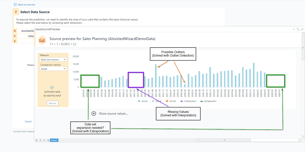
The Source View button views your source data before going through the data preparation process. You can check for missing values or possible outliers at this stage.

When you are finished, click Next.

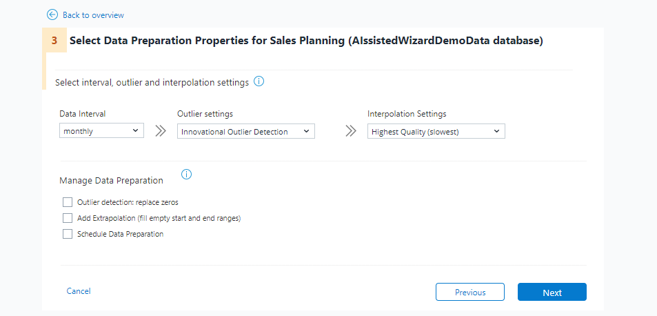
Now you must select the data preparation properties, namely the data interval, outlier and interpolation settings.

Select either a monthly or daily data interval, depending on if there is monthly data or daily data in the cube.

The Outlier Settings options, which find out-of-place or extreme values, are as follows:

• Local Outlier Factor:
  Spots points that stand out compared to their local temporal neighbors. Use when you want to detect anomalies that are unusual in a local time window. Works well with most types of time series as it makes no strong assumptions about input time series (e.g. data does not need to be seasonal). Runs quickly with good quality (good starting point).

• Isolation Forest:
  Outliers in the sequence are easier to isolate because they differ sharply from other time points. Use when you need a scalable method for detecting unusual points in long time series. Works well with numerical time series; no assumptions about seasonality. Fast and scalable, especially for large datasets. Quality is generally good, though it may under-perform on very short or highly seasonal time series.

• Interquartile Range Based Detection:
  Flags points that are far outside the typical range of recent values, by default 25% and 75%. Use when you want a simple method for detecting spikes or dips in a univariate time series. Best for stable time series without strong trends or seasonality. Extremely fast and high quality when data is clean and consistent but may miss context-aware anomalies.

• Z-Score Statistic Based Detection:
  Measures how far a point deviates from the running mean of the series. Use when your time series is roughly stationary and roughly normal in distribution. Works best with stationary time series and normally distributed data. May require normalization and is sensitive to extreme values that can skew the mean and standard deviation. Very fast good quality for clean, symmetric data but may struggle with skewed or seasonal time series.

• Change Point Detection:
  Detects moments when the pattern, mean, or variance of the series shifts. Use when you’re analyzing time series for sudden structural changes or regime shifts. Works well with time series that may contain abrupt changes or transitions. Assumes that changes are meaningful and not just noise. Moderate speed and high quality for detecting structural shifts but not designed for spotting isolated anomalies.

The Interpolation Settings options, which replace missing values and have an “Off” option to disable interpolation, are as follows:

• Gaussian Process Regression Interpolation:
  Models the data as a distribution over functions, using observed points to infer missing values with uncertainty estimates. Use when you need high-quality interpolation with uncertainty quantification, especially for complex or sparse data. Very flexible and powerful. Handles nonlinear patterns well but requires sufficient data. Slower but delivers excellent quality. Ideal for high-stakes or precision-critical applications.

• Linear Regression Interpolation:
  Uses a regression model trained on known data points to predict missing values based on time or other features. Use when you want interpolation that accounts for trends and relationships in the data, not just proximity. Works well with linear trends. Less effective for nonlinear or noisy data. Slower but offers better quality for trend-driven data.

• Linear Approximation with Seasonal Decomposition:
  Separates the time series into seasonal, trend, and residual components, then applies linear interpolation to the non-seasonal parts before recombining. Use when your data has clear seasonal patterns and you want interpolation that respects those cycles. Requires sufficient data to detect seasonality. Works well with periodic or seasonal time series. Moderately fast. Produces high-quality results for seasonal data, but less effective for non-seasonal or irregular series.

• Linear Approximation:
  Estimates missing or intermediate values by drawing straight lines between known data points. It assumes the change between points is linear and smooth. Use when: you need a quick and simple way to fill gaps in time series data or create evenly spaced data points from irregular observations. Works best when the underlying data changes gradually. May not capture complex patterns or sudden shifts well. No assumptions about seasonality or stationarity. Very fast and easy to implement. Quality is acceptable for smooth data or as a baseline method, but may under-perform on highly variable or nonlinear series.

• Spline Interpolation:
  Connects data points with smooth, piecewise polynomial curves, ensuring continuity and smoothness across the entire series. Use when you want to interpolate missing values in data that may have nonlinear trends or require smooth transitions between points. Handles complex patterns better than linear methods. Works well with time series that exhibit gradual changes or curvature. May struggle with very noisy data. Slightly slower than linear interpolation but offers higher quality for smooth, nonlinear data. Good balance between flexibility and stability.

• Polynomial Interpolation:
  Fits a single polynomial curve through all known data points. The curve attempts to capture the overall trend of the data. Use when you need a global approximation and expect the data to follow a smooth, continuous pattern across the entire range. Can be sensitive to noise and overfitting, especially with high-degree polynomials or many data points. Not ideal for long or irregular time series. Slow and prone to instability with large datasets. Quality can be high for small, clean datasets but degrades quickly otherwise.

• Last Observation Carried Forward:
  Fills missing values by repeating the last known observation until a new value appears. Use when you want to preserve recent trends or states, especially in real-time monitoring or categorical data. Best for stable or slowly changing time series. Can misrepresent data if used during rapid changes or long gaps. Extremely fast and simple. Quality depends on data stability; it can be misleading in volatile series.

• Nearest Point Replacement:
  Fills missing values by copying the value from the closest known data point, either before or after the gap, without estimating or smoothing. Use when you need a fast, simple method to fill gaps and the data is relatively stable or categorical (e.g. status flags, labels). Best suited for discrete or slowly changing time series. Can introduce bias or abrupt jumps in highly variable or continuous data. Extremely fast and easy to implement. Quality is low for dynamic data but acceptable for stable or categorical series.

Select the checkboxes to apply additional data preparation management tools. They are:

• Add Extrapolation (fill empty start and end ranges): if your data set does not contain enough data points, extrapolation can help by suggesting values. Check this box to employ this tool.

• Schedule Data Preparation: check this box to automate this data preparation scenario as a task in the Scheduler. The default setting is once per day, but can be changed in the Scheduler tab.

Once you have selected your Data Preparation Properties, click Next.

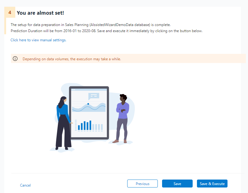
You may now save and execute the data preparation or simply save your settings. Either way, your scenario for this data set will now appear in the overview. Here it can be viewed, modified, and executed at any future point.

Once executed, the data automatically becomes available in the cube and can be implemented in reports and templates.

Updated October 22, 2025